|
|
Air exchange between an enclosure and its surroundings |
The air exchange rate of a room is an important influence on its climate, but it is scarcely ever measured. As a consequence we have kilometres of thermohygrograph charts and terabytes of digital climate records which are no use for diagnostic studies of indoor climate and no longer useful for quality control of the air conditioning.
The definition of air exchange rate is the time, usually expressed in hours, for all the air in a room to be replaced by outside air.
For an air conditioned environment, this is easily quantified as the room volume divided by the flow through the supply duct. This definition assumes forceful displacement of the room air towards the exit duct. This can be described as the Pit and Pendulum concept (after the story by Edgar Allan Poe) - imagine a wall moving through the room sweeping the stale air out at a steady rate with fresh air filling the void behind.
In spaces ventilated by natural leakage through windows, and in showcases, the true air exchange rate is less than the rate of escape of air molecules because as the air within moves out, fresh air infiltrates and continually mixes with the remaining air within the space. Some of the original molecules linger within the room far longer than the exchange rate would indicate, while some of the newly arrived molecules escape quite soon. In principle, the very last stale air molecule will take an almost infinite time to leave the enclosure.
The air exchange rate is often measured by injecting an exotic gas into the space and following the diminution in its concentration over time. It is also possible to use office humans as carbon dioxide generators and follow the decay in the concentration over the weekend. In houses, daytime emptiness allows the same measurement.
Non-human sources of CO2 are readily available in the form of ampoules of compressed gas used to make fizzy drinks, so we don't need to cram a person into a showcase to measure its air exchange rate. Let us open up one of these ampoules within a showcase and follow what happens.
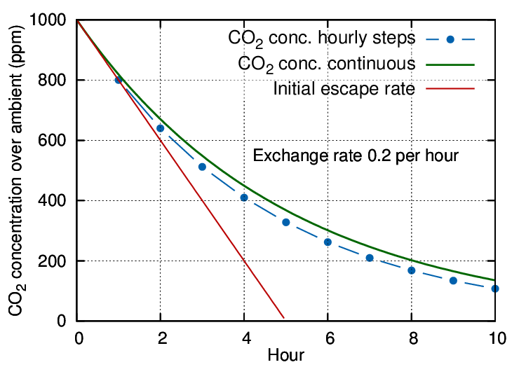
Figure 1: An exchange rate of 0.2 volumes per hour is expressed by the steep, straight line, representing a sweep-through exchange. The dotted line shows the result of hourly calculation of the mixing with infiltrating air. The smooth curve represents a continuous evaluation of the mixing process combined with escape of CO2.
The gas will mix rapidly with the air within the case to give a starting concentration at, say, 1000 ppm over ambient (which is currently about 400 ppm but plays no further part in this simplified discussion). Thereafter, both CO2 and air will diffuse out through small cracks while an equal amount of outside air, mixed with ambient CO2, will move in.
If we let the leakage process run for an hour, the CO2 concentration will have diminished, in this particular case, from the starting 1000 ppm above ambient to 800 ppm above ambient. Mathematically described, the remaining concentration is:
ct = c0 ×(1 − k/n)
Where t is the elapsed time and n is the number of measurements per hour, which is also one in this example. k is the air changes per hour, which is 0.2 in this case.
Entering the second hour, the rate of outward air movement is exactly the same as in the previous hour but the starting CO2 concentration is now lower. This means that fewer CO2 molecules leak out than in the previous hour, though the total number of molecules escaping is the same as in the first hour. After the second hour the remaining concentration of CO2 will be reduced by the same proportion as after the first hour:
ct = c0 ×(1 − k/n) ×(1 − k/n) = c0 ×(1 − k/n)2
The concentration follows the blue dotted trace on the diagram.
In this way a flattening trend develops through successive kinks in the gradient at each measuring interval.
In reality, the dilution of the CO2 proceeds by a continuous process of diffusion out, combined with mixing with infiltrating air. We can calculate a more accurate decay curve by increasing the calculation frequency n, expressed in measurements per hour, in the general equation:
ct = c0 ×(1 − k/n)(n ×t)
The exponent (n × t) represents the total number of calculations performed during t hours.
For a really accurate calculation we have to measure very often, meaning that n, the number of calculations per hour, becomes very large.
This looks like a big calculation, but we can take advantage of a long known simplification for expressions of this kind. Let us put:
q = −n/k
then
k/n = −1/q and n = −qk
Substituting in the decay calculation:
ct = c0 ×(1 + 1/q)(q ×(−kt))
This transformation allows a further simplification: as q becomes large, meaning a very short time interval between calculations, the expression (1 + 1/q)q becomes equal to 2.718 (approximately), which is the magic number e, named by the Swiss mathematician Leonhard Euler.
so now we have:
ct = c0 e−kt
This is a widely applicable equation which describes the diminution with time of a quantity whose rate of decline changes in proportion to its instantaneous value. The usual, and most accurately obeyed, example is radioactive decay, but it also applies, less accurately, to the fall in the level of water in a bucket with a hole in the bottom.
The calculation can be further simplified. At the time of writing we celebrate the 400th anniversary of the invention of logarithms by John Napier in 1614.
The exponent −kt is the logarithm to base e of the concentration ratio ct/c0.
log(ct/c0) = −kt
log(ct) − constant = −kt
This transformation removes the exponent from the equation so that the log of the concentration plotted against time gives a straight line whose gradient is equal to the air exchange rate k. This is the starting rate of the change in concentration of trace gases mixed into the air and is how the exchange rate is usually expressed. However, in most situations this number gives an exaggerated rapidity of change of variable components of air such as carbon dioxide and water vapour.
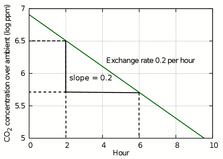
Figure 2: The slope of the plot of log(concentration) against time is straight line whose slope gives the air exchange rate in exchanges per hour.
For calculating leakage of gases from enclosed spaces with a passive climate, such as showcases and boxes, it is more instructive to use the related concept called the half-life. This is the time taken for the concentration to halve, which will be the same as the time for it to halve again. This way of expressing leakage is suitable for predicting the behaviour of showcases with humidity buffers. To illustrate this way of treating air exchange, figure 3 shows the progress of carbon dioxide leakage as ppm on a logarithmic y axis. This is exactly equivalent to plotting the log of c on a linear axis, as in figure 2, but better illustrates the slowness of approach of CO2 or of H2O vapour towards ambient conditions.
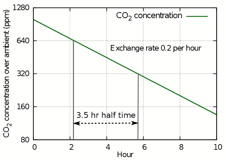
Figure 3: The loss of CO2 shown as a straight line against a logarithmic concentration axis. Each horizontal interval represents a halving of the concentration.
The y axis stretches as the concentration diminishes, so though the concentration line continues with steady downward slope, it never will reach zero because the scale expands to prevent it. Instead we can use the time in hours needed to halve the concentration to express the decay as a half life. In this case the half life is 3.5 hours, while the leakage rate found from the plot of log(ct) is 0.2 volumes per hour, giving a five hour time for total replacement by displacement. The half life is always 0.7 times the exchange rate by displacement.
In practice, the air exchange rate is measured by loss of trace gas in spaces which have mixing in of fresh air as the old leaks out, so the quantity actually measured is the half life. This is then usually converted into the air exchange rate expressed as the exit rate of the starting air at the starting rate. So the quoted air exchange rate is fictional by convention, unless a very refined air displacement air conditioning is installed.
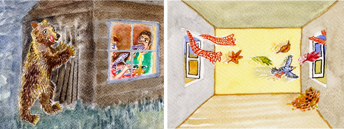
Figure 4: For diffusive processes (left) use half life; for displacement processes (right) use the air exchange rate.
Which is the more useful measure? If there is forceful ventilation, by ducts or by windows arranged on opposite sides of the room, the air exchange rate is appropriate. The half life concept is appropriate for an environment where leakage occurs through random molecular movement through cracks with no distinct streaming flow of gas.
Figure 5 shows a real life example: the record of occupation of the office of a colleague blessed with a varied pattern of work.
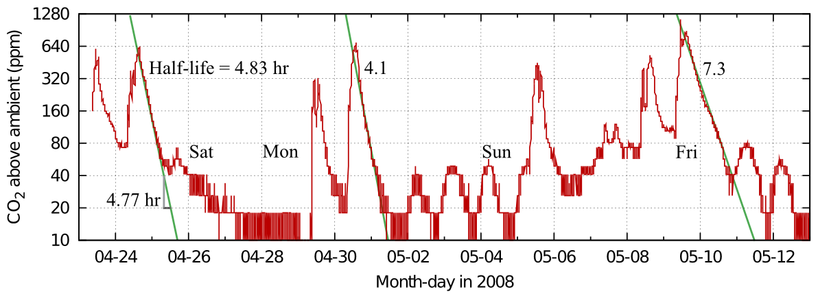
Figure 5: Carbon dioxide dissipation episodes within an office. The half life is quite variable, but slow compared with measurements from ordinary houses. Data from Morten Ryhl-Svendsen.
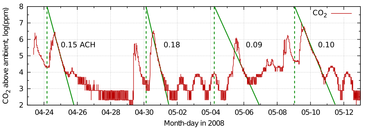
Figure 6: The data from figure 5 plotted on a log scale to give the air exchange rate in air changes per hour.
From this record in figure 5 one can see the variability of the half time in real measurements. The identical graph in figure 6 shows the corresponding exchange rates.
The good linearity indicates mainly diffusive air exchange in this non-air conditioned room.
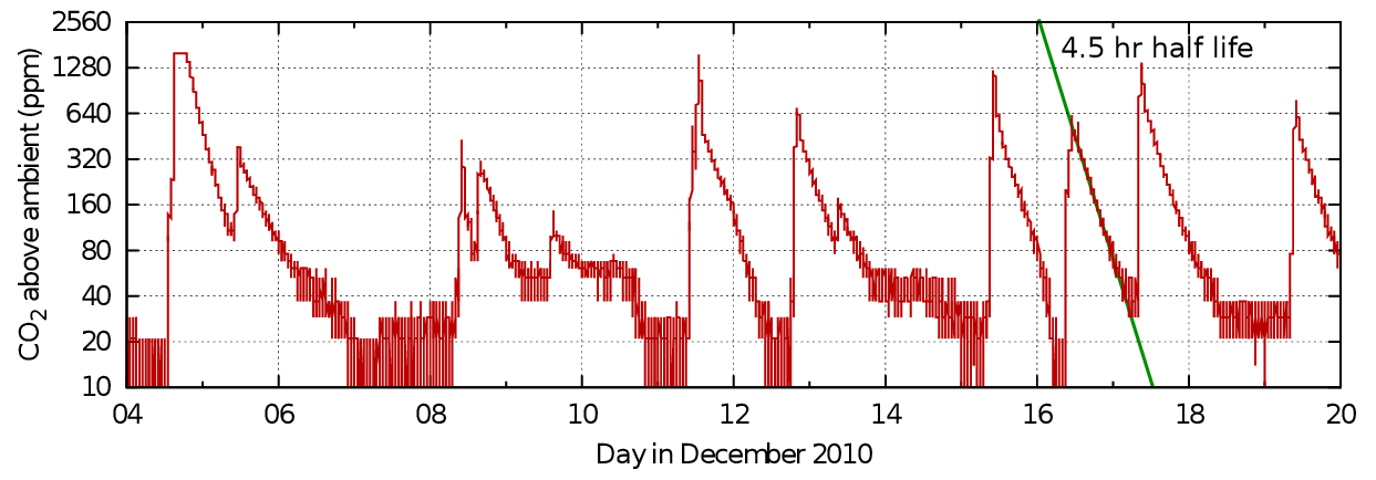
Figure 7: Carbon dioxide dissipation after events in Sondersø church, Denmark. The pattern is similar to that in the single occupation office, though the space is much larger. Data from Morten Ryhl-Svendsen.
Figure 7 is a similar record from a larger enclosure - the gothic church at Sondersø, Fyn, Denmark.
The traces in the graphs from both office and church show good linearity in the mid section of the events but a tendency to concavity towards increasing time. This can be interpreted as an increased loss of carbon dioxide at the peak level, maybe by sorption into the room furniture or more rapid ventilation due to higher than ambient temperature, or windows and doors opened to 'air' the room. At the tail of the decay lines there is a slowing of the approach to the outside value, which can be attributed to outgassing of the previously sorbed gas or to the waning temperature difference and closed doors. Yet another source of a lingering tail in the concentration in a room within a building is leakage between the measured space and other human occupied spaces with higher than ambient carbon dioxide.
Carbon dioxide decay seems to give higher air exchange rates than measurements using rare trace gases found in only minute quantity in the ambient air. The difference can be an order of magnitude. This suggests there is some carbon dioxide sink. It is a water soluble gas and it does react to form bicarbonate ions in solution, perhaps in the surface liquid films which are always present on the surface of materials.

Figure 8: The water vapour concentration indoors is usually higher than outdoors, because of human activities - none of which absorb water vapour.
Another gas which is released by humans is water vapour. This will be strongly absorbed into hygroscopic materials and later released into the space. This process masks the effect of air exchange. However, if we make the simplifying assumption that the hygroscopic material is always in equilibrium with the space around it, we can calculate the course of the decline in concentration after the space is first raised to a high humidity and then exchanges air with a dryer environment.
It is convenient to change the unit of concentration from ppm to relative humidity (RH), because this is the measure which defines the physical properties of absorbent materials. The RH is the actual concentration of water vapour, measured in any concentration unit, divided by the maximum possible concentration at that temperature, which is the limit at which condensation occurs. The RH is a ratio. However, at a constant and uniform temperature, the RH is proportional to the water vapour concentration, so it can be treated in exactly the same way, with the advantage that it directly indicates the physical state, and the quantity of sorbed water, of hygroscopic materials.
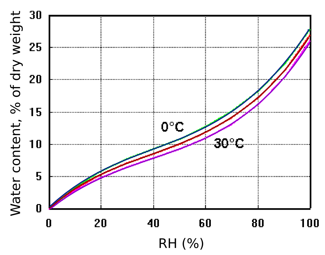
Figure 9: The exchangeable water content of cotton as a function of relative humidity and temperature. The effect of temperature is small. After Urquhart & Williams, 'Absorption isotherm of cotton', J. Textile Inst. (1924) 559-572
Figure 9 shows how cotton cellulose exchanges water with the surrounding space according to the RH, with only a slight influence of temperature. The diagram also shows that cotton contains a large amount of exchangeable water compared with an equal weight of air. One cubic metre of air weighs approximately one kilogram and contains, at room temperature and 50% RH about 10 g of water, equal to the water content of 100 g of cotton cellulose.
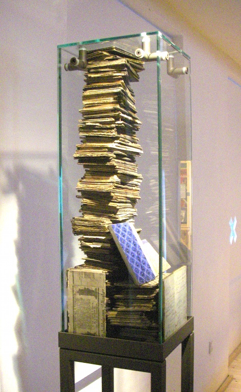
Figure 10: A heavily buffered showcase which will maintain a stable relative humidity for a long time.
Let us inject enough water into a showcase of one cubic metre to raise its RH to 70%, then follow its progress to equilibrium with a surrounding room at 50% RH. If the case were empty, its RH would change exactly as described above for carbon dioxide escape. But suppose that we now put a 200 g book (a typical paperback volume), in the showcase. The paper will contain about 15% of exchangeable water, say 30 g, while the air will contain about 12 g of water vapour. As the RH declines to 50 % through leakage to a dry environment, the air water vapour content will reduce to 8.6 g of water. However, the equilibrium water content of the paper will reduce to 20 g, so it will have released 10 g of water to the air within the case. The paper continuously tops up the water content of the air in the case as its RH diminishes, reducing the rate of decline of RH to a quarter of that experienced by an empty case of the same volume, with the same air exchange rate.
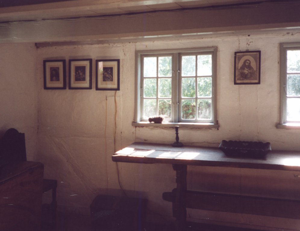
Figure 11: Pictures framed behind glass, hanging in a humid environment.
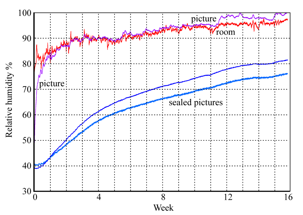
Figure 12: The rise in RH within glazed picture enclosures. Two pictures are sealed with aluminium foil covering the back of the frame, one picture is protected only by permeable card.
Figures 11 and 12 show the buffering process in operation within a set of framed paper images set in a humid environment. The unprotected picture quickly rises to equilibrium with the room RH while the sealed pictures slowly move towards the high ambient RH with a half time of about two weeks. This, however, is not the half time for air exchange, which is much quicker. The delay in reaching equilibrium is mainly due to sorption of water into the paper image and its card mount.
Showcases are often stuffed with absorbent materials to stabilise the RH against leakage to rooms which may be too humid or too dry, sometimes alternating through the seasons. Exotic and expensive sorbents are often used but here we will use paper - to show that specialised buffer materials are not needed in most circumstances.
To calculate how much buffer material to use one must first measure, or guess, the air exchange half-time. Let us take an example of a showcase with a measured half time for inert gas leakage of one day, which is easily attainable. One would like the half-time to equilibrium with the room water vapour concentration to be at least 3 months, say 100 days.
The water vapour emission, or absorption, contributed by hygroscopic materials can be considered equivalent to expanding the case to a larger, fictional volume but keeping the rate of loss of water vapour (and air) the same as in the real case volume. At room temperature, a change of RH from 50% to 40% will change the water content of a space by 1.7 g per cubic metre. This same 1.7 g change of water content will be experienced by about 100 g of paper on being exposed to the same RH step change. So we can say that 100 g of paper within a one cubic metre case imitates an extra cubic metre of humid air and thus effectively doubles the case volume without affecting its leakage rate, expressed in cubic metres per hour. This is the same as saying that it will double the half-life, but only for water vapour.
In this particular case we need to multiply the 'inert' half life by 100, which corresponds to 10 kg of paper per cubic metre. This is not unreasonable: the density of a book is about 500 kg/m3, so only one fiftieth part of the case volume need be sacrificed to buffer material.
If one measures the half-time for a showcase of one cubic metre, using an inert gas such as CO2, one can assume that every 100 g of cellulosic buffer will add one cubic metre of 'virtual' space to the showcase, without changing the rate of loss of water vapour, so there is a proportionate increase in the half-time. Therefore, if you want a showcase which can ride out the dry winter period in a museum in a cold climate, it is easy to calculate how much buffer to add, once one has measured the half-time for air exchange in the empty case - that is the difficult part.
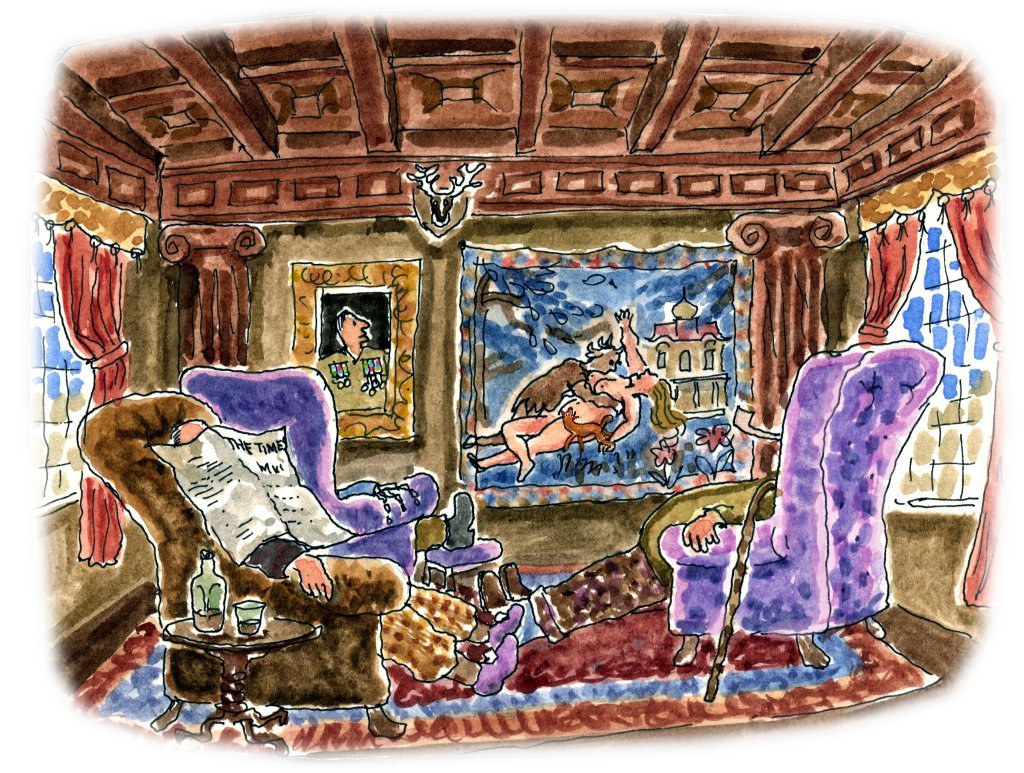
Figure 13: Even a heavily buffered room will usually have an air exchange rate so large that the buffering will only stabilise the room for a few hours.
In a room with larger air exchange rate, the furnishings will provide some buffer action but will not maintain equilibrium with the air, since the rate of diffusion of water vapour through the hygroscopic materials is quite slow compared with the rate of escape of water vapour from the air space. The calculation described above will not work for this situation, because it assumes instant equilibration between the water content of the absorbent material and the RH of the room. The calculation for buffered but leaky spaces is given in detail in a separate article:
www.conservationphysics.org/wallbuff/
padfield_jensen_humidity_buffering_2011.pdf
I thank Morten Ryhl-Svendsen for data and advice.

This work is licensed under a Creative Commons Attribution-Noncommercial-No Derivative Works 3.0 License.